Medical Image Compression Part 1 - Entropy Encoding
There are thousands of different data compression algorithms in existence, many of which you use. Some of the most popular include gzip, JPEG and PNG which are used in almost every web site you visit. You may have also heard of image compression algorithms used in DICOM for medical imaging – specifically JPEG, JPEG-LS, and JPEG 2000. The DICOM standard refers to these image compression algorithms as “Transfer Syntaxes” and each is assigned a unique identifier (or UID). For example, the UID for the JPEG 2000 lossless transfer syntax is 1.2.840.10008.1.2.4.90. The DICOM standard currently supports over 15 different compressed transfer syntaxes and in the past supported another 15 different compressed transfer syntaxes which were not used and retired. You may wonder why there are so many different image compression algorithms and what the difference is between them. That is the focus of this series – to explore the algorithms behind image compression and the associated tradeoffs with a focus on JPEG 2000.
The main objective of compression is to reduce the size of a piece of data. For example, a 512x512 16-bit CT Image is 512KB. A typical CT study may have anywhere between 150 and 2,000 images which therefore is between 75MB and 1000MB in size. When a radiologist reads a study, there can be up to four relevant priors viewed as well, expanding the size of the working set up to 5GB. Newer procedures such as digital breast tomosynthesis and digital pathology can produce studies several GB in size resulting in working sets over 20GB. The trend is clearly towards larger and larger data sets which increasingly stresses storage, memory, network and CPU resources. In addition, there are IT infrastructure and financial implications, which we will explore further in a future post where I will demonstrate the significant cost savings available by using compression in medical imaging.
Let’s explore how DICOM represents images and use a CT as an example. If you look at a typical CT image, you will notice that data is clustered in four ranges of Hounsfield values:
Air: -1,024 to -1,000
Lung: -800 to -200
Soft Tissue: -200 to 400
Bone: 400 to 2,000
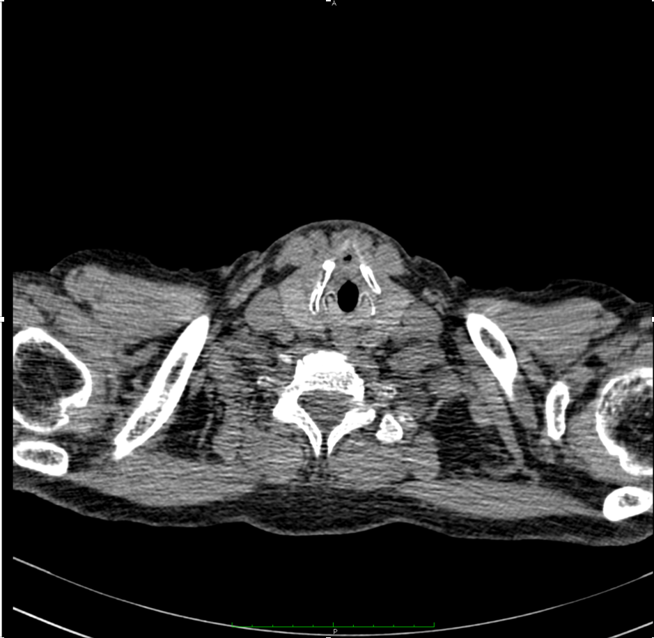
Figure 1: A CT image with three of the four main regions – air (black), bone (white), soft tissue (grey).
CT images have ~3000 unique pixel values (-1024 - 2,000) yet each pixel value is stored in 16 bits (which can represent 65,535 unique values). Clearly, we are using more bits than are needed. This is mainly due to modern CPU architecture which provides access to data on byte (8 bit) boundaries. We cannot store CT pixels in one byte (which can only represent 256 unique values) so we must use 2 bytes per pixel. Some image formats will allow packing of pixels – if a CT only used 12 bits (which is common), we could pack 3 pixels over 4 bytes saving 2 bytes (3 pixels * 12 bits = 36 bits or 4 bytes, 3 pixels * 16 bits = 48 bits or 6 bytes). Bit packing a CT image would therefore achieve a compression ratio of 1.5:1. While bit packing does reduce the size of data, the data itself is not changed at all so it is considered more of a data layout optimization technique rather than an actual image compression technique.
When it comes to lossless data compression, most of the size reduction is achieved by what is called an entropy encoder. An entropy encoder scans the input data symbols (e.g. pixels) and sort them by how often they occur. For example, out of the 262,144 pixels in a 512x512 CT image, the most common value might be -1024 Hounsfield (air pixels) and have around 20,000 occurrences. While the least common value might be +2000 Hounsfield (highly dense bone pixels) and only have one occurrence. After scanning the input data stream and determining which symbols are the most common, entropy encoders produce an output bitstream that uses fewer bits to encode the more common symbols (pixels), more bits to encode the least common symbols (pixels), and a dictionary that maps the entropy encoded symbols to the original symbols. For example:
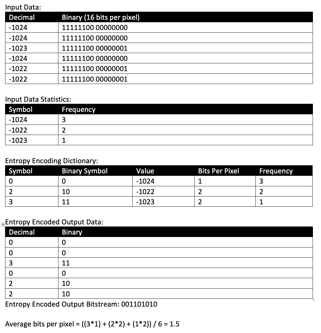
Figure 2: Entropy encoding of 16-bit signed data resulting in output averaging 1.5 bits per pixel. These bits are concatenated (packed) resulting in a compression ratio of 10.6:1 (16/1.5 =10.6)
The most popular entropy encoder is a Huffman encoder which is used by compression algorithms that we use every day – ZIP, JPEG and PNG in particular. Huffman encoding is popular because it is the easiest to implement and provides very good performance. There are other more complex entropy encoders that can be used, JPEG2000 in particular uses an arithmetic encoder which produces slightly better compression ratios than Huffman encoders by about 5%-10%. Arithmetic encoding requires significantly more computation which results in slower encoding and decoding rates. The use of an arithmetic encoder is one of the reasons why JPEG 2000 is slower than other image compression decoders. We will explore performance aspects of JPEG 2000 in more detail in a future post.
Entropy encoders do most of the actual compression and there are only a few entropy encoding algorithms in use, yet as we have all seen there are large differences in the compression ratios they produce. This difference is due to how the data is transformed before it is fed into the entropy encoder and these transformations are what we will explore in a future post.